K-Nearest Neighbours (K-NN) (Kramer 2013) is a widely used algorithm in the field of machine learning and data analysis. It is often used for tasks such as classification and regression. The basic approach of the K-NN algorithm is to identify the \(K\)nearest neighbours of a given data point in a dataset and make a prediction for the given point based on the classifications or values of these neighbours.
Here is a basic description of the K-NN algorithm:
Dataset: First, a dataset is required, which consists of a collection of data points. Each data point has features that define its position in a geometric space.
Distance calculation: To find the nearest neighbours for a given data point, a distance metric is used, often the Euclidean distance. This metric measures the distance between the feature vectors of the data points.
Selection of K: The user must specify a number K, which indicates how many nearest neighbours should be considered. K is a positive integer.
Identification of K nearest neighbours: For a given data point, the K data points are selected from the data set that have the shortest distance to the given point.
Prediction: In a classification task, the class membership of the data point is predicted based on the majority of the K nearest neighbours. This means that the class that occurs most frequently in the K nearest neighbours is selected. In a regression task, the value of the data point is estimated based on the average or weighted averages of the K nearest neighbours.
Evaluation and fitting: The algorithm can be applied to test data to evaluate its performance. Choosing the right K value can have a significant impact on the results, so it is important to choose K carefully.
K-NN is a simple, non-parametric algorithm that does not require explicit model fitting. However, it is sensitive to the choice of K and can be computationally expensive in large datasets or with many features. Nevertheless, it is a useful algorithm for various use cases, especially when the data distribution is non-linear or complex.
In order to apply the K-NN method in an exemplary way, the following question will be examined to find out which influences lead to research teams creating a climate of cooperation characterised by trust to the highest degree. This is a relevant question because it has been repeatedly shown that a climate of cooperation characterised by trust is an important factor for the success of research teams (e.g. Hückstädt 2023).
Data
In the following, the KNN method is tested with cross-sectional data from a large-scale web survey conducted in 2020 as part of the joint project Determinants and Effects of Cooperation in Homogeneous and Heterogeneous Research Clusters (DEKiF) (Hückstädt et al. 2023). The survey focused on the internal cooperation processes of research clusters, on cooperation problems that arise in the course of joint work, and on possible solutions to internal cooperation problems. The target population of the survey was N = 15,595 PIs and spokespersons who have participated in Research Clusters (RC) funded by the German Research Foundation since 2015. The target population included disciplinary and interdisciplinary, large and small (in terms of staff), disciplinary homo- and heterogeneous as well as multi-local RC. The database GEPRIS, which contains information on projects (and project members) funded by the German Research Foundation (DFG), was used to determine the population as well as to collect contact information.
The sample collected consisted of \(n = 5306\) participants from \(n = 948\) RC, of which \(n = 4971\) were PIs and \(n = 335\) were speakers. This corresponds to a response rate of 34 per cent. The sample consisted of 26 per cent female and 74 per cent male participants. The average age of the respondents was \(x = 52.67\) years with a standard deviation of \(SD = 9.52\).
Recoding
We load the DEKiF-data into the workspace and recode the Trust-Variable (problm_9).1 We code as high trust those cases that indicate that the collaboration within their research team is characterised by trust to a high extent, and as no high trust those cases where this is not the case.
As can be seen, in terms of internal trust relationships, DFG teams’ cooperation is similarly often perceived as being characterised by trust to the highest degree as not or less trusting.
Which variables could be responsible for the fact that the cooperation climate is not always perceived as trustworthy to the highest degree?/
Disciplinary heterogeneity
Communication barriers: Different disciplines have different disciplinary cultures. If team members have difficulty communicating in an understandable way, this can affect trust as misunderstandings and miscommunication can occur.
Differences in working methods: Team members from different disciplines may have different ways of working and methods. This can lead to conflict and reduce trust if team members have doubts about the effectiveness or quality of others’ work.
Prejudices and stereotypes: In interdisciplinary teams, prejudices and stereotypes about certain disciplines might occur, which can affect the trust of team members. If members of a discipline are mistakenly seen as less competent, this can reduce confidence in their abilities (Shrum, Chompalov, and Genuth 2001; Hückstädt 2023).
Number of members
Coordination and decision-making: As the number of team members in a team increases, coordination and decision-making can become increasingly complex. Each member may have different ideas, priorities and ways of working, which can lead to conflicts or delays, which in turn reduce the trust relationships among members.
Responsibilities: Each member has responsibility for certain aspects of the project. However, if the number of members in a team is too high, it can be difficult to establish clear responsibilities and ensure that each team member is performing their tasks effectively. Diffusion of responsibility can induce free-rider behaviour, which can also negatively affect trust relationships between members.
Resource allocation: The number of members can also influence the allocation of resources such as research funds, laboratory resources and research staff. If there are too many members, the limited resources risk being shared inefficiently, which can lead to friction and eventually to a loss of trust (Defila, Di Giulio, and Scheuermann 2006).
Frictions
Decisions regarding the distribution of resources or content can lead to conflicts, for example if they are not reached on the basis of consensus. The tensions resulting from unacceptable decisions can lead to a loss of trust in the team if some members are overreached in the allocation of resources without comprehensible justification.
To specify the aforementioned input variables in the context of the K-NN, we use the select() function to select the dichothomised trust variable coded above, as well as the number of subjects in a research team, the number of researchers in a research team, the extent of conflicts arising in the context of resource allocation or content-related decisions.
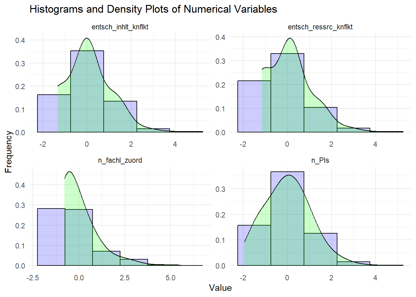
Since K-NN is a distance-based algorithm, the results are affected by the scaling of the input variables. To avoid this, we scale our data in the following and look at the distributions of the input variables using the ggpplot() function.
df_knn <- df_knn %>%mutate_if(is.numeric, scale)df_knn %>%select_if(is.numeric) %>%gather() %>%ggplot(aes(x=value)) +geom_histogram(aes(y=..density..), colour="black", fill="blue",binwidth =1.5, alpha=.2)+geom_density(alpha=.2, fill="green", adjust =3) +facet_wrap(~key, scales ="free")+theme_minimal() +labs(x ="Value", y ="Frequency") +ggtitle("Histograms and Density Plots of Numerical Variables")
Analysis
We import the caret package and set the seed for reproducibility. The trust variable is used as a stratification variable, which means that the proportion of “high trust” and “no high trust” in the variable is kept constant in both the training and the test data set. The argument times is set to 1, which means that the function creates only one partition. The argument p is set to 0.8 so that 80% of the data is used for training the K-NN and 20% for testing the model. Finally, the argument list is set to FALSE so that the function returns a vector of indices rather than a list of data frames.
library(caret)set.seed(123)trainIndex <-createDataPartition(df_knn$trust, times=1, p = .8, list =FALSE)train <- df_knn[trainIndex, ]test <- df_knn[-trainIndex, ]
Im folgenden trainieren wir ein K-NN-Modell unter Verwendung der train()-Funktion des caret-Pakets. Die Funktion train() nimmt verschiedene Argumente entgegen:
trust ~ . specifies trust as output variable, . all other variables in the data set as input variables.
the train data set is specified as the data basis.
as the applied estimation method, the KNN we focused on.
During training, 10-fold cross-validation is used to evaluate the performance of the model. Finally, different values of the tuning parameter ‘k’ are tested, namely 3, 5,7 and 9 as specified by ‘tuneGrid = data.frame(k = c(3,5,7,9))’. The resulting model is stored in an object called ‘knnModel’ and can now be used for further analysis.
The Caret package provides some straightforward and powerful method for assessing models. To calculate the assessment metrics of model performance, it is first important to generate predictions for the trust variable of the test data set. We then use these predictions and the actual values to evaluate the model performance.
Confusion Matrix and Statistics

               Reference
Prediction      high trust no high trust
  high trust           150           106
  no high trust        136           235

               Accuracy : 0.614
                 95% CI : (0.5747, 0.6523)
    No Information Rate : 0.5439
    P-Value [Acc > NIR] : 0.000227

                  Kappa : 0.2154

 Mcnemar's Test P-Value : 0.062295

            Sensitivity : 0.5245
            Specificity : 0.6891
         Pos Pred Value : 0.5859
         Neg Pred Value : 0.6334
             Prevalence : 0.4561
         Detection Rate : 0.2392
   Detection Prevalence : 0.4083
      Balanced Accuracy : 0.6068

       'Positive' Class : high trust
The confusionMatrix() function gives us some important parameters that allow us to evaluate the performance of our model:
Accuracy: The accuracy of the model is .6061, which means that it made 60.61% of the predictions correctly. This is a reasonable performance, which is significantly higher than estimates that would be based on the “No Information Rate”.
Kappa: The kappa value is .199. Kappa is a measure of the agreement between the model’s predictions and the actual values. A high Kappa value close to 1 indicates good predictive performance, a low Kappa value close to 0 indicates poor predictive performance. In this case, our K-NN model can be addressed as poor.
Sensitivity: The sensitivity of the K-NN is 0.5140. The model is therefore able to correctly predict about 51% of the “high trust” cases.
Specificity: The specificity is 0.6833 and further shows that the model correctly predicts approx. 68% of the “no high trust” cases.
Conclusion
The specified model has comparatively good classification strength, but is only slightly better than random in terms of prediction. In summary, therefore, the K-NN model has some predictive power, but there is room for improvement. More imput variables should be specified and different K values tested to see if a different choice of K leads to better performance.
References
Defila, Rico, Antonietta Di Giulio, and Michael Scheuermann. 2006. Forschungsverbundmanagement: Handbuch für die Gestaltung inter- und transdisziplinärer Projekte. Zürich: vdf Hochschulverlag.
Hückstädt, Malte. 2023. “Ten Reasons Why Research Collaborations Succeeda Random Forest Approach.”Scientometrics 128 (3): 1923–50. https://doi.org/10.1007/s11192-022-04629-7.
Hückstädt, Malte, Bernd Kleimann, Monika Jungbauer-Gans, and Deutsches Zentrum Für Hochschul- Und Wissenschaftsforschung (DZHW). 2023. “Quantitative Partial Survey of the ProjectDEKiF.”German Centre for Higher Education Research and Science Studies (DZHW). https://doi.org/10.21249/DZHW:DECQUANT:1.0.0.
Kramer, Oliver. 2013. “K-Nearest Neighbors.” In Dimensionality Reduction with Unsupervised Nearest Neighbors, edited by Oliver Kramer, 13–23. Berlin, Heidelberg: Springer. https://doi.org/10.1007/978-3-642-38652-7_2.
Shrum, Wesley, Ivan Chompalov, and Joel Genuth. 2001. “Trust, Conflict and Performance in Scientific Collaborations.”Social Studies of Science 31 (5): 681730.
Footnotes
See for an overview of the measuring instruments: https://metadata.fdz.dzhw.eu/public/files/instruments/ins-decquant-ins1/$-1.0.0/attachments/Codebuch_Questionnaire_Final.EN.pdf↩︎